Using rSETSe

This vignette walks through a simple analysis shown in the paper The spring bounces back (arXiv:2007.09437), using 5 network classes known as Peels quintet (Peel et al 2018 doi.org/10.1073/pnas.1713019115). The purpose of the vignette is to show you how to go from a collection of networks to a plot summarising their final embeddings.

Setup

The first block, shown below, loads all the necessary packages. use install.packages() if any of the packages are not installed on your machine.

library(rsetse)
library(dplyr)
library(tidyr)
library(ggplot2)
library(purrr)
library(ggraph)
library(igraph)

Peel’s quintet

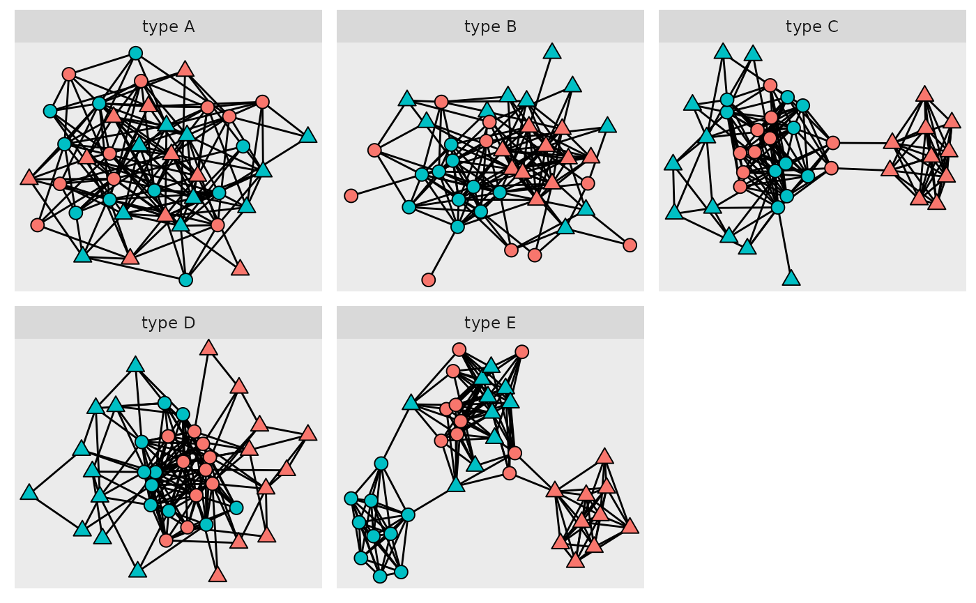
Anscombe’s quartet which showed that figures that were visually very different could have almost identical correlation and other summary statistics. Peels quintet is the graph equivalent of Anscombe’s quartet but for graph/networks. The networks in Peel’s quintet have two groups of nodes which are broken up into two subgroups. All the networks have the same number of node, edges, connections within and between groups. However, the connections between subgroups change producing very different networks even though they appear identical using traditional network metrics (for more information see the paper by Peel et al).

the rSETSe package has a function that generates each of the 5 types of Peels network. The code chunk below shows 1 example of each class of the quintet starting with type A on the left and ending with type E on the right. It is clear that networks

#This is a bit of a contorted way to get 5 networks into the same plot as 
#igraph::union does not also merge attributes
set.seed(1263)
peels_networks <- 1:5 %>%
  map(~generate_peels_network(LETTERS[.x]) %>%
        #The nodes in all the networks are numbered 1:40, this line ensures
        #each class has distinct node names
        set.vertex.attribute(., "type", value = paste("type", LETTERS[.x])) %>%
        set.vertex.attribute(., "name",
                             value = as.numeric(get.vertex.attribute(., "name"))+(.x-1)*40) %>%
      #The networks are going to be joined into a single network so need to be converted into a
      #list of dataframes
      igraph::as_data_frame(., what = "both")
      ) %>%
  #the list is now two elements long and made up of a edge and vertex part
  transpose() %>%
  #join the elements from each part of the list into dataframes
  map(~bind_rows(.x)) %>%
  {graph_from_data_frame(d = .$edges, directed = FALSE, vertices = .$vertices)}



ggraph(peels_networks) +
  geom_edge_fan()+
  geom_node_point(aes(fill = class, shape = grepl("1", sub_class)), size=3) +
  scale_shape_manual(values=c(21, 24)) +
  guides(fill = "none", shape = "none") +
  facet_nodes(~type, scale = "free")

# Creating lots of networks

First we will generate 10 examples of each class of the Peel’s quintet.

set.seed(4563)
all_peels <- LETTERS[1:5] %>% map(~{
  
  peel_type <- .x
  
  out <- 1:10 %>% map(~{
    
    generate_peels_network(peel_type)
    
    })
  
})

#Embedding lists of networks

Then we will embed all graphs in the list using setse_auto, however before the graph can be embedded they need to be prepared for setse using one of the setse preparation functions prepare_categorical_force or prepare_continuous_force. The prime purpose of these functions make ensure that the force variable has a mean of 0, creates a spring constant k if necessary, creates the node distance variable. As the Peel’s quintet is a network of two node classes A and B we will use prepare_categorical_force.

Once the networks have been prepared they can be embedded. After embedding the graph type and id number is added on to the embeddings data to ensure we catagorise the graph easily.


#The first map cycles though each of the graph types from A to E
all_embeddings <- 1:5 %>% map(~{

temp_list <- all_peels[[.x]]
  
node_type = LETTERS[.x]
#The inner map embeds each of the 10 networks of that type
out <- 1:10 %>%
  map(~{
    id_number <- .x
    g <- temp_list[[.x]]
    embeddings_data <-g%>%
      #standard edge preparation is fine as k is included in the dataset
      prepare_edges() %>%
      #k has already been generated by the generate_peels_network function 
      prepare_categorical_force(., node_names = "name",
                     force_var = "class") %>%
      #The system is considered converged when the static force is 1/10000 of 
      #absolute sum of the force exerted by all the nodes
    setse_auto(force = "class_A", tol = sum(abs(vertex_attr(., "class_A")))/10000) 
    #create the aggregated node details
    #embeddings_data$node_details <- create_node_details(g, embeddings_data)
    embeddings_data$node_details <- create_node_edge_df( embeddings_data)
    
    element_names <- names(embeddings_data)
    #add the id data onto each df in the list
    embeddings_data <- 1:length(embeddings_data) %>%
      map(~embeddings_data[[.x]] %>% mutate(type = node_type,
                         id = id_number))
    
    names(embeddings_data) <- element_names
    
    return(embeddings_data)
  })

return(out)
  
})

#the list of embedding networks is then transposed and all the dataframes 
#representing the networks are made into a list of 5 dataframes using bind_rows
all_embeddings <-all_embeddings %>%
  flatten() %>%
  transpose() %>%
  map(bind_rows)

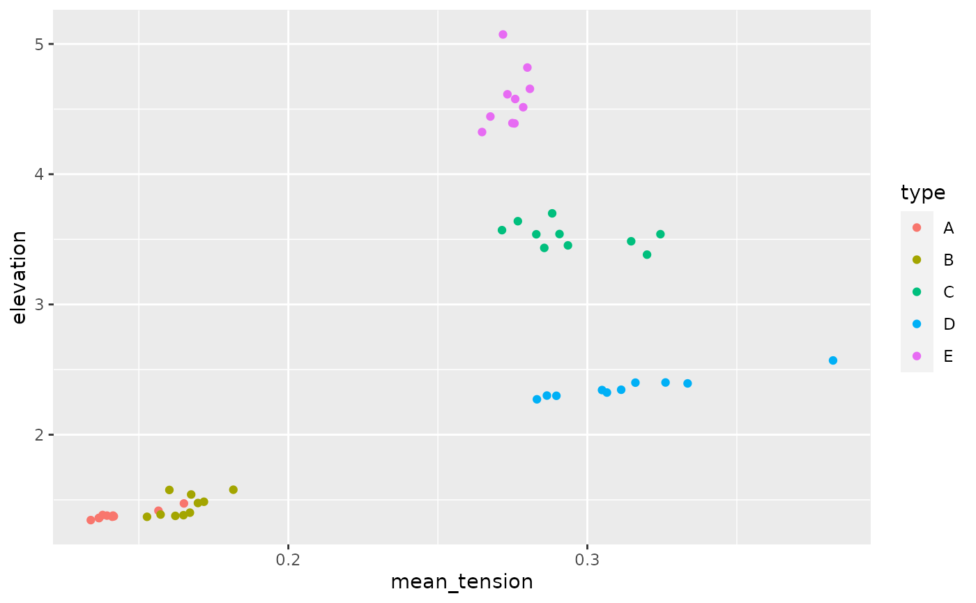
Aggregate to graph level and plot

aggregate the node level details up to whole graph level and plot the results




all_embeddings$node_details %>%
  group_by(type, id) %>%
  summarise(mean_tension = mean(tension_mean),
            elevation = sum(abs(elevation))) %>%
  ggplot(aes(x = mean_tension, y = elevation , colour = type)) + geom_point()

We can see that the networks in peels quintet are clearly distinguishable using SETSe.

Analysing multiple networks

Using rSETSe

Setup

Peel’s quintet

Aggregate to graph level and plot